The one number that decides whether an outbreak explodes

One number decides whether an outbreak fizzles out or engulfs a country: if each case infects more than one other person on average, the outbreak grows without limit. If it infects fewer than one, the outbreak dies. That number is called $R_0$ (said "R nought"), and everything else — the terrifying exponential, the reassuring flattening, the vaccination target on the evening news — falls out of it with GCSE maths.

In this paper we build the whole story from one case. We will derive the exponential phase, discover why exponentials must bend, recover the famous herd immunity formula, and finish with a genuinely uncomfortable twist that the headline version of the story always leaves out.

I. What R nought actually measures

$R_0$ is defined as the average number of people that one infected person passes the disease to, in a population where everybody is susceptible. That last clause matters enormously, and it is the hinge on which the rest of this paper turns.

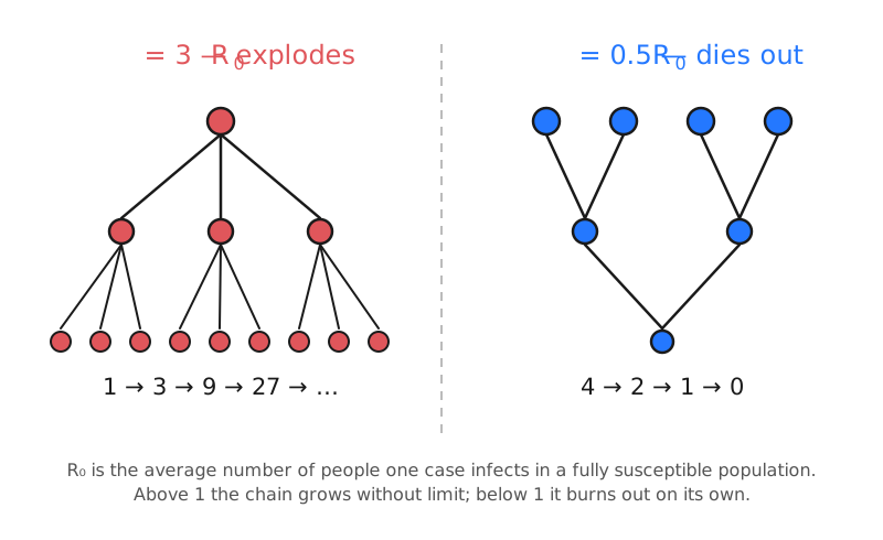
The logic is a chain. One case makes $R_0$ cases. Each of those makes $R_0$ more. If $R_0 > 1$ each generation is bigger than the last, and the chain compounds. If $R_0 < 1$ each generation is smaller, and the chain runs out of people to infect and stops on its own — no intervention required.

So what are the real values? Seasonal influenza has a median estimated $R$ of about 1.28 — each case infects roughly one and a quarter others [2]. Measles is the usual poster child for the other extreme, with a figure of 12–18 quoted in essentially every textbook and news article.

And here we should be honest, because this is where the famous version of the story starts to fray. When Guerra and colleagues went looking for the evidence behind that 12–18 range, they screened 10,883 citations, kept 18 studies, and extracted 58 separate estimates of measles $R_0$. Their conclusion was blunt: the estimates "vary more than the often cited range of 12–18" [1]. The number everyone repeats is not a constant of nature. $R_0$ is not a property of a virus alone — it is a property of a virus in a population, and it depends on how crowded, how connected, and how well-ventilated that population is. A measles $R_0$ measured in a dense unvaccinated community simply is not the $R_0$ of a sparse rural one.

We will use $R_0 = 3$ from here on. It is a plausible mid-range respiratory value, and it makes the arithmetic clean.

II. One case, sixty days, 800,000 infections

Let us give our disease a generation time of 5 days: the average gap between someone catching the disease and passing it on. With $R_0 = 3$, every 5 days the number of new cases triples.

Start with one case on day 0 and count generations. After $n$ generations, the number of new cases is:

$$\text{new cases in generation } n = 3^n$$

Sixty days is $60 \div 5 = 12$ generations. So on day 60, the number of new cases is:

$$3^{12} = 531{,}441$$

To get the total number of people infected so far we add up every generation, $1 + 3 + 9 + \cdots + 3^{12}$. This is a geometric series, and there is a tidy trick for summing it: call the total $S$, multiply it by 3, and subtract. Every term cancels except two:

$$S = \frac{3^{13} - 1}{2} = \frac{1{,}594{,}323 - 1}{2} = 797{,}161$$

From a single case, 60 days. Under 800,000 infections — nearly a million people — in two months, from one person, with a disease that only infects three others per case. That is the whole horror of exponential growth in one line, and it is the same arithmetic that puts an absurd quantity of rice on a chessboard or folds a sheet of paper to the moon.

It is worth noticing how modest the ingredients are. Nothing here is exotic. Three infections per case, five days apart, and the number ran away from us.

III. Why every exponential must bend

Now push our formula one generation further, to day 65:

$$S = \frac{3^{14} - 1}{2} = 2{,}391{,}484$$

If our country holds 1 million people, the model has just confidently infected 2.4 million of them. The model is broken, and the way in which it is broken tells us exactly what we left out.

Our chain assumed every one of the three people a case meets is susceptible. Early on that is nearly true — with a handful of cases in a million people, almost everyone they meet has never had the disease. But once a serious fraction of the population has already been infected, some of those three contacts are people who have already had it. Those infections simply do not happen. The transmission is wasted.

So we define the effective reproduction number. If $s$ is the fraction of the population still susceptible, then only a fraction $s$ of a case's would-be infections land on someone new:

$$R = R_0 \times s$$

This one line is the engine of the entire epidemic. At the start $s \approx 1$ and $R \approx R_0 = 3$. As people are infected, $s$ falls, so $R$ falls with it — not because anybody did anything, but because the disease is running out of fuel.

To watch it happen, we simulated a population of 1,000,000 with $R_0 = 3$ in Python, tracking each generation. In each round, every susceptible person gets a chance to escape every currently infectious person; the survivors carry on to the next generation. Here is what the simulation gives:

• Day 40 — 99.7% still susceptible, so $R = 2.99$. Total infected: 9,769.
• Day 50 — 97.1% susceptible, $R = 2.91$. Total infected: 83,001.
• Day 55 — 91.7% susceptible, $R = 2.75$. Total infected: 220,424.
• Day 60 — 78.0% susceptible, $R = 2.34$. Total infected: 483,806.
• Day 65 — 51.6% susceptible, $R = 1.55$. Total infected: 765,763.
• Day 70 — 23.4% susceptible, $R = 0.70$. Total infected: 899,469.
• Day 80 — 6.7% susceptible, $R = 0.20$. Total infected: 939,072.

Look at day 60. Our runaway exponential claimed 797,161 infections; the honest simulation says 483,806. And look at what happened to $R$: it fell from 3 to 2.34 without a single intervention. By day 70 it has dropped below 1 and the epidemic is dying — of natural causes.

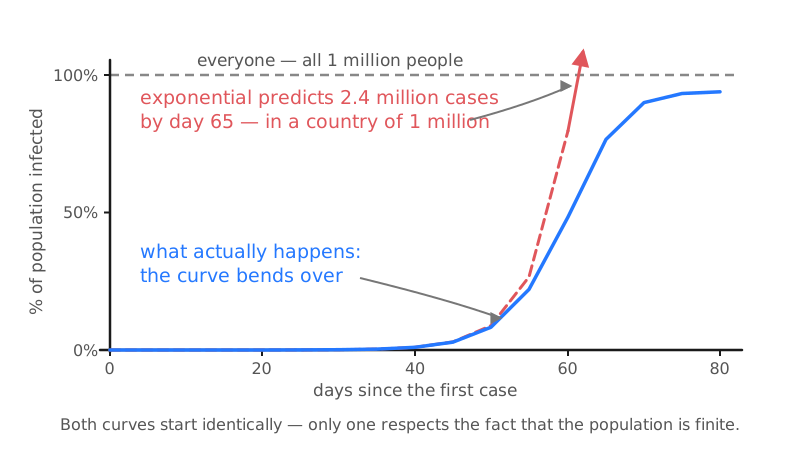
The result is the famous S-curve (or logistic curve): a slow start that looks like nothing is happening, a violent middle that looks like an exponential, and a flattening top. Crucially, the top is not flat because anyone succeeded. It is flat because the susceptibles ran out.

IV. Why you never have to reach everybody

We now have everything we need for the number that dominated public conversation for two straight years.

The epidemic grows while $R > 1$ and shrinks while $R < 1$. So the turning point — the peak — is exactly where $R = 1$. Setting $R_0 \times s = 1$ and rearranging:

$$s = \frac{1}{R_0}$$

That is the fraction that must remain susceptible. So the fraction that must be immune is everyone else — and this is the herd immunity threshold:

$$\text{HIT} = 1 - \frac{1}{R_0}$$

For our $R_0 = 3$ disease, $1 - \frac{1}{3} = 66.7\%$. Once two thirds of the population are immune, each case infects fewer than one other person on average, and the outbreak shrinks even though the disease is still circulating and plenty of susceptible people remain. That is the whole idea: you never have to reach everybody. The immune majority absorbs enough transmissions to break the chains for the minority.

Run the formula across our real values:

• Seasonal flu, $R_0 = 1.28$: threshold $1 - \frac{1}{1.28} = 21.9\%$.
• Our example, $R_0 = 3$: threshold $66.7\%$.
• Measles, taking $R_0 = 15$: threshold $1 - \frac{1}{15} = 93.3\%$.

This single fraction explains a fact that otherwise looks like fussiness: why measles campaigns chase 95% coverage while nobody demands that for flu. It is not that measles is more feared. It is that $1 - \frac{1}{15} = 93.3\%$, so a measles-free population has almost no margin. Vaccinate "only" 80% against measles and the effective $R$ is $15 \times 0.2 = 3.0$ — still firmly above 1, and measles comes back. The same 80% against our $R_0 = 3$ disease gives $3 \times 0.2 = 0.6$, comfortably below 1. High-$R_0$ diseases are unforgiving in a way that is purely arithmetic.

V. The twist: epidemics overshoot

Here is the part the tidy version leaves out, and it is the best thing in this paper.

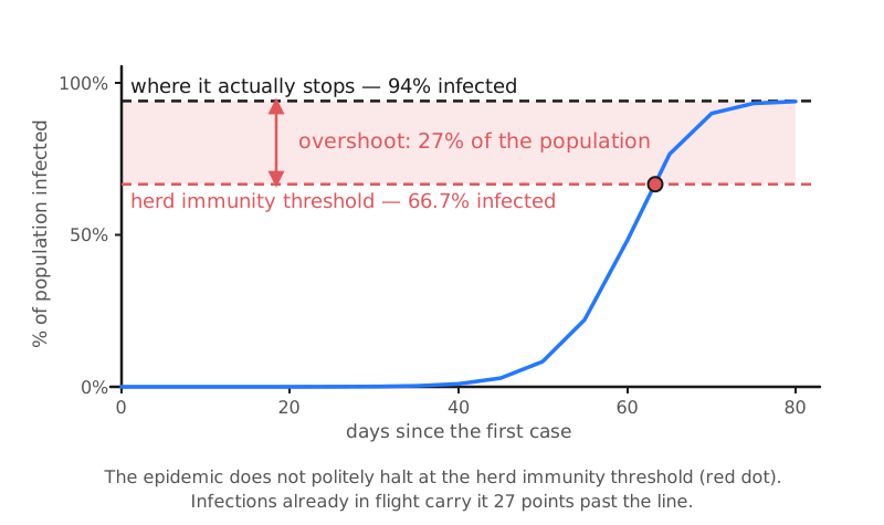
We just showed that once 66.7% of our population is immune, $R$ drops below 1 and the epidemic starts shrinking. It is tempting to conclude that the epidemic therefore stops at 66.7%. Look again at the simulation: it finishes with 94.0% of the population infected.

It sailed 27 percentage points past the threshold. Over a quarter of a million extra people, in our million-person country, infected after herd immunity had already been achieved.

Why? Because $R < 1$ does not mean "no more infections". It means "each case infects fewer than one other". At the moment the threshold is crossed, there is still a huge army of currently-infectious people mid-flight, and every one of them still infects somebody — just slightly fewer than one somebody. The epidemic decays rather than stopping dead, and the sum of that decaying tail is enormous. It is momentum: the epidemic coasts well past the line before friction brings it to rest.

We can check this independently, without any simulation at all. There is a classical result — the final size equation — which says the eventual fraction infected, $z$, satisfies:

$$1 - z = e^{-R_0 z}$$

Solving numerically for $R_0 = 3$ gives $z = 0.940$. Our step-by-step simulation and this century-old formula agree to three decimal places, which is a reassuring sign that we have not fooled ourselves.

And the overshoot carries a real moral. Reaching herd immunity by simply letting an epidemic run does not cost you the threshold — it costs you the threshold plus the overshoot. For $R_0 = 3$, that is 94% infected rather than 67%. Reaching the same threshold by vaccination costs you only the 67%, because vaccination raises immunity without a cloud of infectious people already in the air. The two routes to the same immune fraction do not have the same bill.

VI. What our model ignores

One number, $R_0$, really does decide it. Above 1 and the chain compounds; below 1 and it dies. Our $R_0 = 3$ disease reached 797,161 cases in 60 days on paper, 483,806 in an honest simulation, and eventually infected 94.0% of everyone — despite needing only 66.7% immune to turn the corner.

We should be clear about what we simplified. We used one fixed generation time where reality has a spread; we assumed everybody mixes with everybody at random, when real contact networks are clustered and people mostly meet the same few dozen people; and we held $R_0$ constant, when in a real epidemic behaviour changes the moment people get frightened — which is itself a way of pushing $R$ down that our model cannot see. Networked and age-structured models soften the peak and lower the overshoot. And as we saw at the outset, even the input number is shakier than its confident textbook range suggests [1].

But the skeleton survives all of that. Exponentials bend because susceptibles run out; the threshold is $1 - \frac{1}{R_0}$; and an epidemic left alone will always overshoot it. The maths is GCSE. The consequences are not.

---

References:

[1] Fiona M. Guerra, Shelly Bolotin, Gillian Lim, Jane Heffernan, Shelley L. Deeks, Ye Li and Natasha S. Crowcroft, "The basic reproduction number (R0) of measles: a systematic review," The Lancet Infectious Diseases (2017). PubMed

[2] Matthew Biggerstaff, Simon Cauchemez, Carrie Reed, Manoj Gambhir and Lyn Finelli, "Estimates of the reproduction number for seasonal, pandemic, and zoonotic influenza: a systematic review of the literature," BMC Infectious Diseases 14:480 (2014). Open access

[3] Roy M. Anderson and Robert M. May, Infectious Diseases of Humans: Dynamics and Control (Oxford University Press, 1991).

Note: Our simulation assumes a homogeneously mixing population, a fixed 5-day generation time and a constant $R_0$. Real epidemics have none of these. The qualitative conclusions — exponential growth, the bend, the threshold and the overshoot — are robust; the exact percentages are not.